Tutorial

This tutorial will guide you through the first steps of getting started with the topotoolbox for python. For further examples regarding the functionality and use cases of different functions/classes refer to the provided examples.

Installation

Before you can use this tutorial the make sure to have the topotoolbox installed as per the installation guide.

Working with this file

Feel free to download this notebook so can follow these first steps in an interactive way.

• Downloading the notebook: curl -o tutorial.ipynb https://raw.githubusercontent.com/topotoolbox/pytopotoolbox/main/docs/tutorial.ipynb or wget -O tutorial.ipynb https://raw.githubusercontent.com/topotoolbox/pytopotoolbox/main/docs/tutorial.ipynb

• You’ll need to install Jupyter Notebook to run this file: pip install notebook

• To plot the DEMs you’ll also need matplotlib installed: pip install matplotlib

• To run the notebook: jupyter notebook

Working on a first DEM

Before you can actually use the topotoolbox package, it has to be imported. Since we want to plot the DEMs we will also import matplotlib.pyplot.

import topotoolbox as topo
import matplotlib.pyplot as plt

To automatically download one of the example files, the function load_dem() is used. To find out which files are available, use get_dem_names(). After the DEM has been created, you can view it’s attributes by using GridObject.info().

print(topo.get_dem_names())

dem = topo.load_dem('taiwan')

print('\nAttributes of the dem:')
dem.info()

['kedarnath', 'kunashiri', 'perfectworld', 'taalvolcano', 'taiwan', 'tibet']

Attributes of the dem:
name: taiwan
path: /home/runner/.cache/topotoolbox/taiwan.tif
rows: 4181
cols: 2253
cellsize: 90.0
bounds: BoundingBox(left=197038.4533204764, bottom=2422805.9007333447, right=399808.4533204764, top=2799095.9007333447)
transform: | 90.00, 0.00, 197038.45|
| 0.00,-90.00, 2799095.90|
| 0.00, 0.00, 1.00|
crs: EPSG:32651

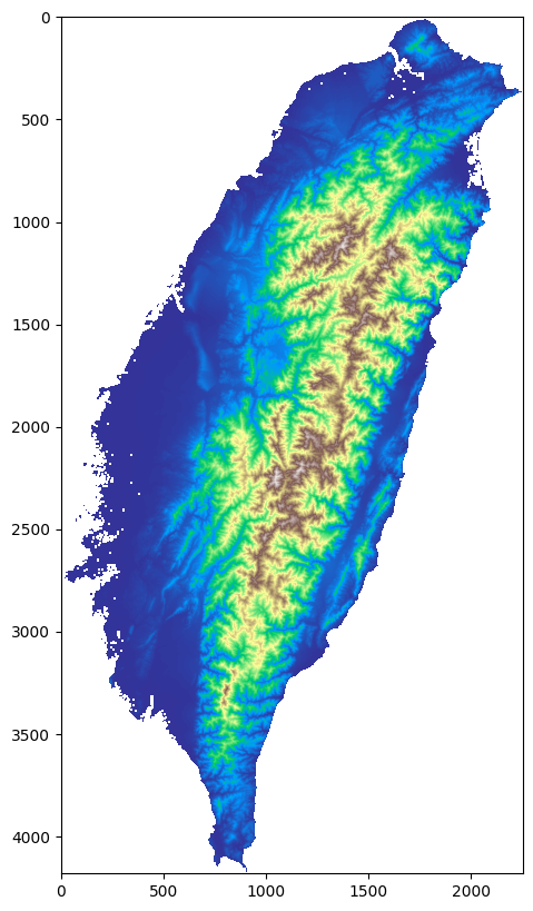
When plotting with matplotlib, the DEM behaves like a np.ndarray. So you’ll just have to pass it as an argument.

If you want to increase the resolution of the plot, increase the dpi value

fig, ax = plt.subplots(figsize=(10, 10), dpi=100)

ax.imshow(dem, cmap='terrain')
plt.show()